The OEE dashboard turned green this quarter. Availability is up, changeovers are faster, the improvement team got a well-earned thank-you. Then the monthly finance review came, and EBITDA hadn’t moved. Nobody lied and nobody made a calculation mistake. The gains were real. They just happened in the wrong place.
In 24 years of working with production lines, planning and process engineering, I have seen this pattern more often than any other: efficiency improves locally, but the plant’s throughput stays the same, so the money never shows up. This article explains why, and gives you a simple method to point every OEE project at the profit line.
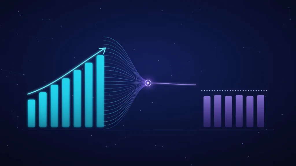
Line OEE vs. bottleneck OEE
OEE (Overall Equipment Effectiveness) multiplies three factors: availability × performance × quality. The idea comes from Seiichi Nakajima’s work on Total Productive Maintenance (TPM). It is a very good measure of how well one asset uses its planned time.
The trouble starts when we average it. A line has one step that sets the pace for everything: the constraint, or bottleneck. One hour lost there is one hour lost for the whole plant. One hour saved anywhere else is usually saved only on paper. That is the core message of Eliyahu Goldratt’s The Goal.
The surprising part: the bottleneck is often not the station with the worst OEE. OEE is a percentage of a machine’s own ideal speed. A fast machine with poor OEE can still out-produce a slow machine with excellent OEE. So don’t look for the lowest number on the dashboard. Look for:
- Queues and WIP: work piles up in front of the constraint.
- Starved and blocked time: stations after the constraint wait for parts; stations before it get blocked or are pushed to over-produce.
- Effective output: ideal rate × OEE, in good units per hour. The lowest of these is your pace.
If you need a step-by-step way to confirm it, use my earlier article How to find and open a production bottleneck with data and its printable Bottleneck Finder checklist (PDF).
From OEE to EBITDA: the chain that matters
An OEE gain reaches the profit line only when it travels along this chain:
Two ideas from throughput accounting (developed by Goldratt and later by Thomas Corbett) make this chain practical:
- Throughput (T) = sales price − truly variable cost (mainly materials). Labour and overhead usually don’t change when you make one more unit, so they belong in operating expense.
- T per bottleneck minute. This tells you which minutes are worth the most, and which SKUs to protect when the constraint is full.
And one honest condition: the extra units must be sold. If the market, not the plant, is the constraint, more output just becomes inventory.
A short loss tree: asset → shift → product → reason
A loss tree turns “OEE is 72%” into “we lose this much money, here, for this reason.” Keep it to four levels:
- Asset: start at the bottleneck. Track other stations, but don’t chase them.
- Shift: the same machine often behaves very differently on different shifts (handovers, breaks, staffing, material supply).
- Product (SKU): changeovers, cycle times and scrap rates depend on what you run.
- Reason: the three OEE losses. Availability (breakdowns, changeovers, starved or blocked), performance (minor stops, slow cycles) and quality (scrap and rework, especially after the bottleneck).
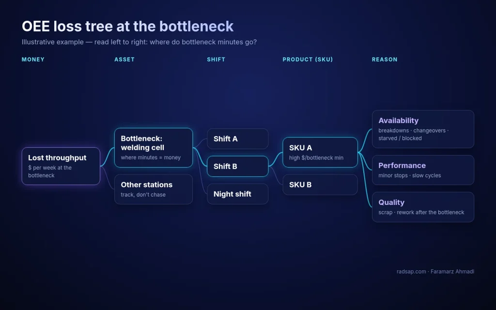
Worked example (illustrative)
A simple line with three stations runs 16 planned hours a day:
| Station | Ideal rate (units/h) | OEE | Effective output (good units/h) |
|---|---|---|---|
| Cutting | 100 | 60% | 60 |
| Welding (bottleneck) | 60 | 80% | 48 |
| Assembly | 90 | 70% | 63 |
Cutting has the worst OEE, and welding the best. Yet welding is the bottleneck, because it has the lowest effective output. The line can only ship about 48 units per hour.
Project A: improve cutting OEE from 60% to 75%
Cutting can now make 75 units/h. The line still ships 48. If cutting runs freely, up to 27 extra units per hour pile up in front of welding, about 430 units in a 16-hour day. By Little’s Law (WIP = throughput × lead time), 430 extra units at 48 units/h add roughly 9 hours of waiting time. Result: higher OEE, more WIP, more cash tied up, no extra profit.
Project B: improve welding OEE from 80% to 86%
- Welding output rises from 48 to 51.6 units/h, so +3.6 units/h × 16 h = +57.6 units/day.
- Assembly scraps 3% after welding, which leaves about 55.9 good units/day.
- With throughput of $15 per unit ($40 price − $25 materials), that is about $838/day, or roughly $17,600/month over 21 working days.
If operating expense doesn’t change and the market takes the units, almost all of that reaches EBITDA.
Bonus: scrap after the bottleneck is the most expensive scrap
Every unit scrapped in assembly already used 1.25 minutes of welding, which is the plant’s scarcest time. Cutting assembly scrap from 3% to 1% adds about 2% × 51.6 × 16 ≈ 16.5 good units/day (≈ $248/day) without touching the bottleneck at all.
Which SKU deserves the bottleneck?
| SKU | Price | Materials | Throughput / unit | Welding time | Throughput / bottleneck minute |
|---|---|---|---|---|---|
| A | $40 | $25 | $15 | 1.25 min | $12.0 |
| B | $55 | $35 | $20 | 2.0 min | $10.0 |
SKU B has the bigger margin per unit, but SKU A earns more per bottleneck minute. When the constraint is full, that is the number that decides the mix and the schedule. Always check customer commitments first, of course.
A practical 5-step method
- Confirm the real constraint. Use queues, WIP and starved/blocked time, not the lowest OEE. (The Bottleneck Finder checklist helps.)
- Measure bottleneck OEE every shift, with reason codes. Tag each loss by asset, shift, SKU and reason, and build the loss tree.
- Price the minutes. Calculate throughput per bottleneck minute for each SKU, then rank losses by money, not by minutes.
- Fix in money order and subordinate the rest. Protect the bottleneck from starving (a small buffer in front), shorten its changeovers, cover breaks, cut scrap after it, and release material at the bottleneck’s pace. Don’t reward OEE gains elsewhere that only build WIP.
- Close the loop with finance. Every week, connect bottleneck good units → throughput $ → schedule attainment → change in operating expense and inventory. If the money doesn’t show, check demand and the next constraint.
Want to apply this in your plant?
If your OEE projects are succeeding but the P&L isn’t moving, I can help you find the real constraint, build the loss tree from your own data, and connect it to throughput and EBITDA.
Contact me Read: find your bottleneck with data
Sources
- Goldratt, E. M. & Cox, J. (1984). The Goal: A Process of Ongoing Improvement. North River Press.
- Goldratt, E. M. (1990). The Haystack Syndrome: Sifting Information Out of the Data Ocean. North River Press. (Throughput, inventory and operating expense.)
- Corbett, T. (1998). Throughput Accounting. North River Press.
- Nakajima, S. (1988). Introduction to TPM: Total Productive Maintenance. Productivity Press. (Origin of OEE.)
- Little, J. D. C. (1961). A proof for the queuing formula: L = λW. Operations Research, 9(3), 383–387. doi:10.1287/opre.9.3.383